Imagen principal: Alvin – un vehículo de ocupación humana (VOH) sumergible diseñado para permitir la recolección de datos a profundidades hasta 6,500 m por debajo de la superficie del océano. Imágen principal cortesía de John Magyar, Caltech.
Autores: Daniela Osorio-Rodriguez, Kyle S. Metcalfe, Shawn E. McGlynn, Hang Yu, Anne E. Dekas, Mark Ellisman, Tom Deerinck, Ludmilla Aristilde, John P. Grotzinger, and Victoria J. Orphan
Tal vez un fin de semana en tu vida, te encuentres apilado en un vehículo todoterreno a las 6 de la mañana con otros siete estudiantes, registrando intermitentemente el dron de un profesor de geología demasiado entusiasta cuya clase tomaste para llenar un requisito de tu programa. Si es así, en ese vehículo con certeza se pronunció la proclamación “el presente es la clave del pasado”. Un estudio reciente conducido por Daniela Osorio-Rodriguez y colaboradores epitomiza el poder de esas palabras.
Featured Image: Alvin – a submersible Human Occupancy Vehicle (HOV) designed to allow data collection at depths up to 6,500 m below the ocean surface. Featured image courtesy of John Magyar, Caltech.
Authors: Daniela Osorio-Rodriguez, Kyle S. Metcalfe, Shawn E. McGlynn, Hang Yu, Anne E. Dekas, Mark Ellisman, Tom Deerinck, Ludmilla Aristilde, John P. Grotzinger, and Victoria J. Orphan
Maybe one weekend in your life, you found yourself piling into an SUV at 6 AM with seven other students, intermittently registering the drone of an overenthusiastic geology professor whose course you took to fulfill a degree requirement. If so, in that vehicle, the proclamation that “the present is the key to the past” was certainly uttered. A recent study conducted by Daniela Osorio-Rodriguez and collaborators epitomizes the power of those words.
Authors: Sofia Baliña, María Laura Sánchez, Irina Izaguirre, Paul A. del Giorgio (2023)
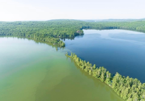
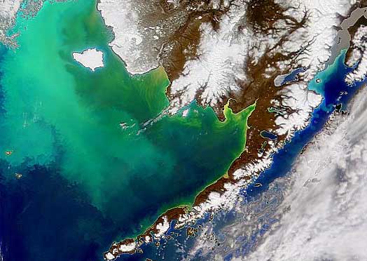
Imagine some of the most dynamic, ecologically important lakes in the world…. you are picturing a deep, wide lake, not something knee deep and murky, or so full of aquatic plants you can’t see the bottom, right? Well, perhaps you should; while they don’t always make the most inviting swimming holes, small, shallow lakes have an outsized importance in the cycling of carbon and other nutrients through the landscape.
Shallow depths tend to lead to warmer temperatures and more concentrated growth of algae and aquatic plants, not always the most desirable features for recreation. But what these lakes might lack aesthetically, they make up for with a massive contribution to the global carbon cycle. Combine the abundance of small lakes with a tendency for frequent mixing of the water column, and high rates of organic input from the surrounding watershed and small lakes pack a big punch in terms of cycling nutrients, including carbon, through pathways in both the water and lake bottom sediments.
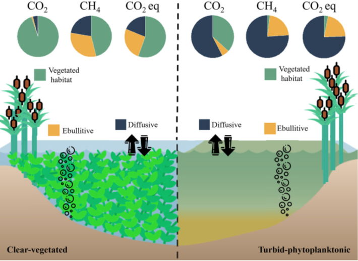
These carbon cycling power houses are tricky to pin down because they can operate in what scientists call two different ‘stable states’: a murky, turbid state, dominated by algal growth that blocks the sunlight from reaching the bottom, and a clearwater state where plants anchored in the lake bottom sediments are dominant. A number of natural events, including floods, droughts, or changes in surrounding vegetation can lead to a ‘flip’ between states. Human activity can lead to a ‘flip’ as well, for example, in the Pampean Plains of Argentina, agricultural practices have added excess nutrients to the system, which tends to push lakes toward the murky, turbid state. The two lake states not only look different from the surface, but also have important differences in rates of photosynthesis, burial of organic material, and circulation in the water.
Knowing the importance of small lakes to global carbon cycling, a team in Argentina did a detailed investigation on how the different states impact carbon cycling and green house gas emissions. By monitoring sets of turbid and clear shallow lakes in the Pampean Plains over the course of a year, they found important seasonal differences in rates of carbon dioxide (CO2) diffusion into and out of water column, and in the flux of methane (CH4) from lake bottom sediments.
Through monitoring instrumentation suspended in the air above the lakes, as well as measurements taken in the water and sediments, researchers were able to observe weather-driven seasonal changes. The biggest differences were between winter and spring: cold, clear lakes tended to act as CO2 source. When the lakes warmed up, they started to move gas from the water into the atmosphere and became carbon sinks, while turbid lakes did the opposite.
Figure 3 from Baliña et al. (2022) showing the different pathways and relative ratios for carbon flow in clear-water, vegetated lakes (on the left) compared to more green, or turbid, lakes with heavy algal growth on the right. In total, the total greenhouse gas emissions (or CO2 equivalents) for both lake states was similar, but came from different pathways in the lake.
Over an annual cycle, clear lakes had as much as 5 times the CO2 emissions to the atmosphere as compared to turbid lakes, mainly attributed to the vegetation. Turbid lakes, however, had a higher annual emission of CH4. On balance, the two groups of lakes had roughly the same total contribution to green house gas fluxes, but the seasonal variability and differences in carbon pathway are important to understand as we continue to learn more about these dynamic ecosystems and how they change over time.
Authors: Sam J. Purkis, Hannah Shernisky, Peter K. Swart, Arash Sharifi, Amanda Oehlert, Fabio Marchese, Francesca Benzoni, Giovanni Chimienti, Gaëlle Duchâtellier, James Klaus, Gregor P. Eberli, Larry Peterson, Andrew Craig, Mattie Rodrigue, Jürgen Titschack, Graham Kolodziej, Ameer Abdulla
Today, scientists are turning to extreme ecosystems on Earth to understand how life evolved on Earth and how life might be on other planets. One such alien place exists in the darkness of the ocean. It’s an extreme ecosystem where even fish think twice before entering. Brine pools are well known for being ‘death traps’ – extremely toxic, and any organism (with a few exceptions) that swims into them dies instantly. They are lakes of hypersaline water present on the ocean floor that are so dense that Remotely Operated Submersible Vehicles (ROVs) float on them!
Featuring image: Titan’s atmosphere is rich in organic molecules, but we still don’t know if there is life on Saturn’s icy moon. With JWST and the coming generation of telescopes, we will be able to observe the atmospheres of exoplanets. Is there a way to search for life on these distant worlds? NASA/JPL, public domain (CC0).
Authors: M. A. Thompson, J. Krissansen-Totton, N. Wogan, M. Telus and J. J. Fortney
Visiting and exploring exoplanets for extraterrestrial life still belong to the realm of science fiction. However, the coming generation of telescopes will enable us to look into the atmospheres of exoplanets and search for possible biosignatures, chemical compounds that could indicate the presence of life.
Searching for life on a planet is not a trivial task. Since the first Mars landing in 1976, scientists still search for recent or ancient traces of life. It becomes even more difficult on planets that we cannot directly visit. The next telescope generation will enable us to observe the atmosphere of distant planets remotely. Are there ways to find evidence of life in a planet’s atmosphere? A new study suggests that the freshly launched James Webb Space Telescope (JWST) could help us to search for life on other worlds.
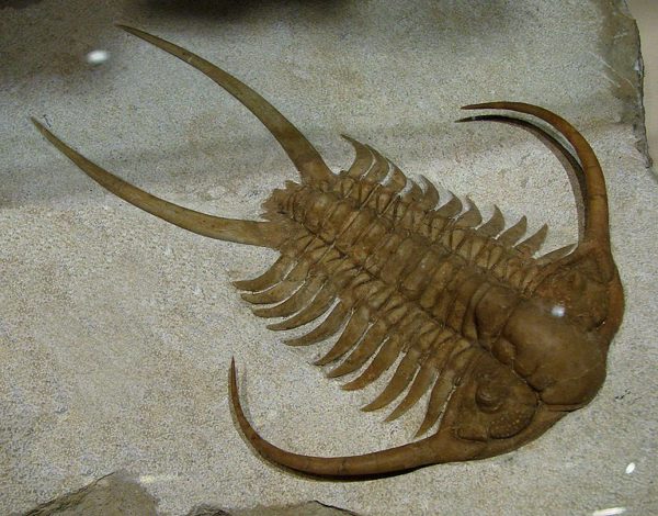
Featured image: This is a Trilobite fossil from Volkhov river, Russia. Trilobites were marine arthropods which went extinct at the end of Permian period. CC BY-SA 3.0 via Wikimedia commons
Authors: William J. Foster, J.A. Hirtz, C. Farrell, M. Reistrofer, R. J.Twitchett, R. C. Martindale
What if I told you that an extinction event occurred In Earth’s history that dwarfs the demise of dinosaurs? This turbulent period dawned 252 million years ago, during the Late Permian period. The largest volcanic eruptions in the history of our planet began in now what is known as Siberia. The eruptions spewed out millions of cubic kilometers of lava, enough to bury an area the size of United States under a mile thick layer of rock!
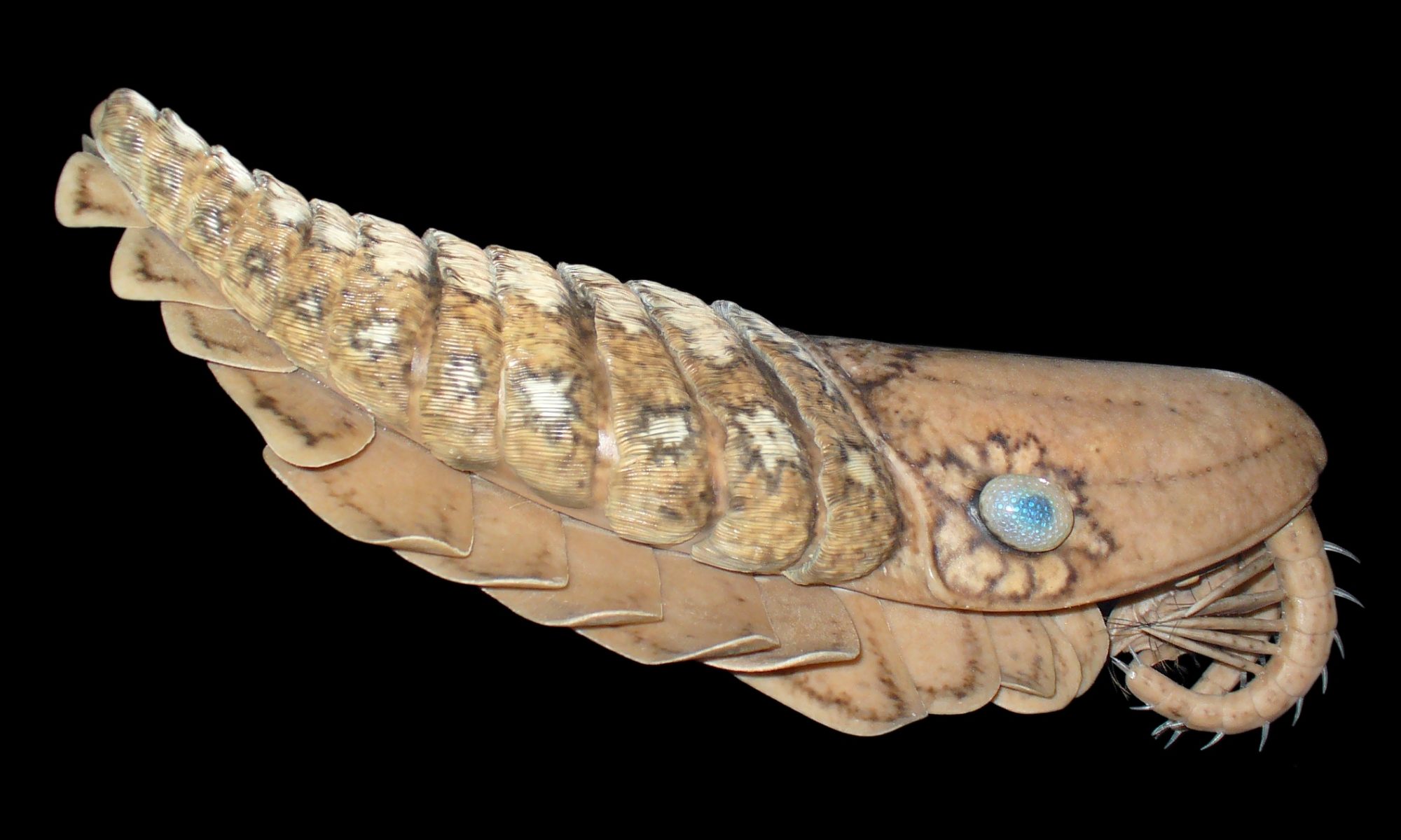
Featuring image: Life on during the Ordovician period looked very different then today. Animals like anomalocarididaes were very common, but many species vanished at the end of the Ordovician. A new study sheds light on the first mass extinction event. Model created by Espen Horn, photo: H. Zell, Creative Commons (CC BY-SA 3.0).
Authors: N. P. Kozik, B. C. Gill, J. D. Owens, T. W. Lyons and S. A. Young
As mountains rise and continents fall apart, it not only changes the face of the Earth, but also drastically affects its inhabitants.
Earth’s biosphere was disrupted by several mass extinction events, often connected to great changes in large geologic cycles. These times of great disasters were also a chance for pioneers and led to great evolutionary leaps. A new study suggests that the oldest of the known major mass extinctions during the Ordovician was caused by a change in climate and the ocean’s circulation system.
Authors: Craig R. Walton, Oliver Shorttle, Frances E. Jenner, Helen M. Williams, Joshua Golden, Shaunna M. Morrison, Robert T. Downs, Aubrey Zerkle, Robert M. Hazen, Matthew Pasek
With a swift strike, a match bursts into flame. Life, like the flame, burst into existence almost 4 billion years ago, and as with the sparking of the match, phosphorus was a key ingredient. Phosphorus, element 15, is at the center of energy production in cells, forms cell walls, and provides the backbone for DNA.
Article: Why productive lakes are larger mercury sedimentary sinks than oligotrophic brown water lakes
Authors: Martin Schütze, Philipp Gatz, Benjamin‐Silas Gilfedder, Harald Biester
Advisories and outreach campaigns have worked for years to help us understand how the fish we eat impacts the amount of hazardous mercury we consume. Mercury is present in the environment naturally in several forms, but consumption advisories warn against methyl-mercury. This substance not only moves throughout the aquatic ecosystem, but bio-accumulates, or increases in concentration, as it moves higher in the food chain. But the size of the fish is not the only influence on its mercury levels – it may also matter where it lives.
Most mercury in lakes is initially deposited from the atmosphere. These levels vary regionally, influenced by things like weather patterns and local industry. Mercury is also deposited on land, though, and it can eventually leach and erode from soils, moving through surface and groundwater into local lakes. Researchers have known for some time that the vegetation and soil types in the watershed can influence mercury influx to lakes; for example, coniferous trees generally take up more mercury from the atmosphere than deciduous trees, making the forest litter and, eventually, the organic rich layers of forest soils more concentrated in mercury in coniferous forests.
A recent German study compared mercury levels in two sets of lakes, looking at everything from surrounding vegetation and topography to local weather patterns, and found that previously observed findings held up; mercury levels were higher in leaf litter and organic soils than other surrounding sediments, and higher in areas with more coniferous vegetation. However, when the authors undertook mathematical modelling to balance the input of mercury from atmospheric deposition and local erosion to the outflow, the numbers didn’t add up the same way in all the lakes.
The difference, they documented, was in the productivity of the lakes. Algae scavenge mercury from the water column and, when they die and sink, take the mercury along. This leads to mercury deposition in the lake sediments. By comparing measurements of mercury in the water column, in accumulated sediments on the lake floors, and in sediment ‘traps’ that collect sediment as it is falling through the water column, the researchers showed that large algal blooms significantly increase the transport of mercury from the water column into lake sediments. In a set of forested, alpine lakes that were low in nutrients and had few algal blooms, the monitoring data showed that most of the mercury inputs were eventually lost to a combination of river outflow, re-emission to the atmosphere, and sediment burial. In lakes with higher nutrient loads and more common algal blooms, a similar input of mercury was translated into a much higher flux to the lake sediments, which they traced to the concentration of mercury in the algal organic matter.
The high rate of mercury delivery to lake sediments, especially in very productive lakes, may be bad news for fishing. The high rate of organic matter input to the sediment also leads to a low-oxygen environment which can spur the bacterially-mediated chemical process that turns mercury into the methyl-mercury form. When it is released and recycled from the sediments, it works its way up the food chain. Lakes in many parts of the world are seeing increased algal growth from warmer temperatures and higher nutrient input, and the resultant highly-visible algal blooms may have a significant impact on the invisible movement of hazardous mercury to consumers at the top.
Authors: Kirsten Poff, Andy Leu, John Eppley, David Karl and Edward DeLong
Cells from blooms of phytoplankton, or tiny plants, can enhance carbon flux all the way down to the deepest parts of the ocean. The authors of this recent study measured the amount of carbon in sinking particles deep in the ocean at a station near Hawaii. Over the course of three years, scientists identified three time periods of unusually high carbon flux, or transport, at this depth, and found that the organisms that made up the sinking particles were significantly different between high flux events and the rest of the time period. The data showed higher abundances of surface-dwelling microorganisms, including phytoplankton, contributing to these particles during high-flux events.

